Driving the GODOT game engine with OSC messages

Problem?

Note: I've tested this code with a very recent version of GODOT compiled from source code. Your mileage may vary.

In interactive art installations, an often used protocol to communicate between computer processes is the open sound control (OSC) protocol. Despite the name "sound" in OSC, the protocol is actually completely general purpose. In my opinion a game engine like the godot engine would benefit tremendously from built-in support for the OSC protocol because it opens up the engine to creative uses outside the gaming domain. On of my own use cases is to visualize in real-time musical events that are algorithmically generated (also in real-time) in supercollider.

The GODOT development team, despite several requests from users, chose not to support OSC directly and provide a high-level networking interface which they feel is more appropriate for their game engine (but which only works with their game engine). 

As a result, some users have attempted to write add-on modules using the GdNative C++ add-on mechanism to extend the GODOT engine. Such modules often have the drawback of limited portability and requiring users to set up a C++ building environment. In addition, the API that needs to be used by the add-ons could be changing drastically between GODOT versions. 

Therefore, I was hoping to find a more portable solution. Luckily GODOT also provides some lower level networking classes, which allow third-party developers to add some support for unsupported protocols.

OSC is typically a thin layer on top of UDP networking (sometimes TCP is used, but most often UDP is chosen for reasons of performance), and so it should be possible to add a simple OSC implementation in GDScript directly.

Note: to make sense of this blog post, you need to have a little bit of working knowledge about the GODOT game engine, at the minimum, you need to know what nodes are.

Will it perform super fast? 

Probably not. But often you don't really need to send tons of data over the network to drive your visualization. Think about optimizing your data streams.

Will it be easy to use?

I think it is extremely easy to use. But feel free to try it out and judge for yourself.

How can I use it?

Glad you ask. Here's the big picture:

To the root note of our GODOT sketch (usually a Node2D for 2d games, or a Spatial for 3d games), I attach a script that monitors the network for incoming OSC messages. The OSC messages are decoded and automatically dispatched to child nodes who requested to be kept informed about certain incoming messages.

Consider an example of a Node2D rootnode (which I renamed to RootNode in the IDE) with a Sprite child node. In the script attached to the Sprite, I only have to express my desire to be kept up-to-date about incoming OSC messages, e.g. here's the complete script for a sprite that can change position by receiving a /set/xy OSC message.

extends Sprite

func _ready():
   get_tree().get_root().get_node("RootNode").register_dual_arg_callback("/set/xy", get_node("."), "set_xy")

func set_xy(x, y):
   self.position.x = x
   self.position.y = y

This means that when the Sprite is instantiated, it registers itself with the root node ("register_dual_arg_callback"). It tells the root note that it wants its function "set_xy" to be called whenever a "/set/xy" OSC message is received over the network with two arguments (x and y) which in this example then are used to set the sprite position. There's also a register_single_arg_callback for functions that expect only one value (and nothing prevents you from adding more variants).

This simple code suffices to ensure that from now on, this particular Sprite will automatically react to incoming OSC /set/xy messages by updating its position.

E.g. in an environment that supports sending OSC message like supercollider, I can run the following snippet to update the sprite position:

(

b = NetAddr.new("127.0.0.1", 4242); // create the NetAddr
b.sendMsg("/set/xy", 650, 200);

)

The godot sketch automatically reacts to the OSC message by updating the sprite xy position to 650, 200, exactly what we requested the system to do by registering a callback. Needless to say the OSC message could perfectly come from another computer, tablet or phone (e.g. from the TouchOsc app or from Open Stage Control).

The value 4242 is the port number on which the root node is listening for incoming OSC messages. In the proof of concept code it's hardcoded to 4242, but you are of course free to change it or to make it configurable.

Ahm, ok. Show me this magic code that goes into the root node then?

Note: the code in this section is obsolete, and replaced by the code in part 2 of this article: https://technogems.blogspot.com/2021/11/driving-godot-game-engine-with-osc.html

Well... it's not the prettiest code (it's a proof of concept - things like IP address and port are hardcoded, but should be simple to change). It works well enough for me at the moment (but I've only done some basic experiments so far). In case I run into trouble, I may need to revisit the details. If you run into trouble, please let me know what happened and how you solved it (or just explain the problem and we can discuss to see if we can find a solution).

Here's the code I put in the root node. For now it only supports parsing integer, float, string and blob OSC messages. In the future maybe also OSC bundles and some other data types could be added, but even with only this simple subset of OSC supported, the possibilities are already endless.

Note that the call to OS.set_low_processor_usage_mode may not be portable across all platforms, but it's probably not strictly needed to make the system work (but don't take my word for it, I'm not at all experienced with GODOT on platforms other than linux).

The code for registering callbacks and dispatching probably can be made a bit more general, and there could be support for pausing, resuming and stopping reacting to OSC notifications but for demonstration purposes what I have here should suffice.

extends Node2D

var IP_CLIENT
var PORT_CLIENT
var PORT_SERVER = 4242 # change me if you like!
var IP_SERVER = "127.0.0.1" # change me if you like!
var socketUDP = PacketPeerUDP.new()
var observers = Dictionary()

func register_single_arg_callback(oscaddress, node, functionname):
 observers[oscaddress] = [1, node, functionname]
 
func register_dual_arg_callback(oscaddress, node, functionname):
 observers[oscaddress] = [2, node, functionname]
 
func _ready():
 OS.set_low_processor_usage_mode(true)
 start_server()
 
func all_zeros(lst):
 if lst == []:
  return true
 for el in lst:
  if el != 0:
   return false
 return true

func _process(_delta):
 if socketUDP.get_available_packet_count() > 0:
  var array_bytes = socketUDP.get_packet()
  #var IP_CLIENT = socketUDP.get_packet_ip()
  #var PORT_CLIENT = socketUDP.get_packet_port()
  var stream = StreamPeerBuffer.new()
  stream.set_data_array(array_bytes)
  stream.set_big_endian(true)
  var address_finished = false
  var type_finished = false
  var address = ""
  var type = ""

                # parse osc address
  while not address_finished:
   for _i in range(4):
    var addrpart = stream.get_u8()
    if addrpart != 0:
     address += char(addrpart)
    if addrpart == 0:
     address_finished = true
    

                # parse osc type list 
  while not type_finished:
   for _i in range(4):
    var c = stream.get_u8()
    if c != 0 and char(c) != ",":
     type += char(c)
    if c == 0:
     type_finished = true

  # decode values from the stream
  var values = []
  for type_id in type:
   if type_id == "i":
    var intval = stream.get_32()
    values.append(intval)
   elif type_id == "f":
    var floatval = stream.get_float()
    values.append(floatval)
   elif type_id == "s":
    var stringval = ""
    var string_finished = false
    while not string_finished:
     for _i in range(4):
      var ch = stream.get_u8()
      if ch != 0:
       stringval += char(ch)
      else:
       string_finished = true
    values.append(stringval)
   elif type_id == "b":
    var data = []
    var count = stream.get_u32()
    var idx = 0
    var blob_finished = false
    while not blob_finished:
     for _i in range(4):
      var ch = stream.get_u8()
      if idx < count:
       data.append(ch)
      idx += 1
      if idx >= count:
       blob_finished = true
    values.append(data)
   else:
    printt("type " + type_id +" not yet supported")

  if observers.has(address):
   var observer = observers[address]
   var number_args = observer[0]
   var nodepath = observer[1]
   var funcname = observer[2]
   if number_args == 1:
    nodepath.call(funcname, values[0])
   elif number_args == 2:
    nodepath.call(funcname, values[0], values[1])
    
func start_server():
 if (socketUDP.listen(PORT_SERVER) != OK):
  printt("Error listening on port: " + str(PORT_SERVER))
 else:
  printt("Listening on port: " + str(PORT_SERVER))

func _exit_tree():
 socketUDP.close()

Compared to the misery of adding, compiling, maintaining, porting, ... a GdNative module, I think this is pretty acceptable (at least for my use cases).

Making an arpeggiator in supercollider with patterns

Problem

Given some notes as input, generate a pattern making use of those notes. When the input changes, the generated pattern should also change. Most keyboards and synthesizers provide simple arpeggiators, but we'll be using supercollider which allows for generating the most complex patterns imaginable including generation of chords, polyphony, introducing random variations, etc
Code for the final piece of code in this post can be found on sccode.org: http://sccode.org/1-5cr

Approach

How can we convert a list of notes to an interesting arpeggio? Different possibilities exist, but we'll be using one of the more powerful abstractions available to supercollider users: the pattern system.

Patterns act as a kind of template for generating events, and events can be played to create sounds. This sounds exactly like what the doctor prescribed.

A simple example to get started

First let's assign some midi notes to a variable ~n:

~n = [60, 64, 67]; // c major chord

If you, like me, prefer to reason in note names instead, you can install the Panola quark:

Quarks.install("https://github.com/shimpe/panola");

Then you can write the following instead (it's a bit longer but, hey,  at least with readable note names):

~n = Panola("c4 e4 g4").midinotePattern.asStream.all;

Our task is to define a pattern that uses the notes in ~n and builds from them a simple arpeggio. So, given the input notes [c4, e4, g4] instead of playing simply the notes [c4, e4, g4] we'll generate a more interesting arpeggio [c4, g4, e4, g4]. When the input notes change to e.g. [c4, f4, a4] the arpeggio that is generated should change to [c4, a4, f4, a4].

(
s.waitForBoot({
    var arp = Pbind(
        \instrument, \default,
        \midinote, Plazy {
            var n0, n1, n2;
            ~n = ~n ?? [Rest(1)];
            n0 = ~n[0] ?? Rest(1);
            n1 = ~n[1] ?? ~n[0];
            n2 = ~n[2] ?? ~n[0];
            Pseq([n0, n2, n1, n2])
        },
        \dur, Pseq([1,1,1,1].normalizeSum*2)
    );
    if (~player.notNil) { ~player.stop; };
    ~player = Pn(arp).play;
});
)

This code requires some explanation:

• s.waitForBoot is a construct I use in pretty much every supercollider sketch I make. It will start the supercollider sound server if it wasn't started yet.
• Once the server is booted, the function that is passed to waitForBoot is executed. This function defines a pattern (also known as Pbind) "arp" and plays it.
• The full power of Pbind is available (meaning that you could e.g. generate midi events and send them to a hardware instrument), but for demo purposes we just instantiate the supercollider default instrument. This should generate some sound even if you don't own any fancy hardware (after all, supercollider is also a sound synthesis language and therefore very capable of generating its own sounds). Instantiating the default instrument is accomplished by specifying the key-value pair \instrument, \default in the Pbind.

Plazy is a filter pattern that allows to calculate a new supercollider pattern using a function.

In addition to selecting an instrument, we also need to generate the notes to be played. Remember that ~n is the input note list. First we try to extract the first 3 notes from the input note list. These are the notes that we will use to rearrange into our arpeggio.

The line ~n = ~n ?? [Rest(1)] checks if variable ~n is defined already (actually it checks if ~n is nil). If it is not defined, it is assigned a list of input notes consisting of a single Rest. Then I introduce some variables n0, n1, n2 to denote the first, second and third note in the input list respectively. It may happen that the input list contains fewer than 3 notes (e.g. if you initialize the ~n variable from midi input from a hardware device, someone might play a 2-note chord instead of a 3-note chord). In that case we don't want our code to crash. If the first note is missing, I replace it with a Rest. If the second or third notes are missing, they are replaced with the first note.

The function passed to Plazy returns a Pseq that generates our arpeggio consisting of the first, third, second and third input note: n0, n2, n1, n2. Pseq is a pattern that generates successive notes. By default the complete list of notes will be repeated once and then the pattern stops.

To generate an arpeggio we are not limited to only generating notes. We can also generate durations, volumes, legato-staccato, and a bunch of other properties. All these can be derived from the input note list, or they can be completely independent from them if so desired. In this first example, let's just give all notes equal duration and keep all other properties to their default values. Specifying durations in a pattern is done by using the \dur key.

I want the complete arpeggio to be finished in 2 beats, so I specify 4 (because there are 4 notes) equal relative durations of 1 and then normalize the values to make their sum == 2.

Finally, we need to stop any previous instances of the pattern that may be playing, and make our pattern start. This happens in the lines

if (~player.notNil) { ~player.stop; }; // call stop if not stopped already
~player = Pn(arp).play;

Note the use of the Pn pattern, to make our arpeggiator repeat indefinitely.

As soon as you redefine the ~n variable to a new value, the pattern (but only after the previous instance was completely finished) will use the new values in ~n and generate a new arpeggio built from the new notes, so e.g. while the pattern is playing, try evaluating the following lines one by one, listening how it changes the arpeggio.

~n = [60, 64, 67 ];

~n =[ 60, 65, 69 ];

~n =[ 59, 65, 67 ]; 

Exercise: adapt the code to make an arpeggio based on the first four notes of a list of input notes.

Exercise: adapt the code to use different durations for different notes

Fancier patterns

The simple arpeggio we generated above is already more complex than what many synthesizers and keyboards can do, but supercollider being supercollider this is just the tip of the iceberg available to us.

We can generate multiple patterns from a single list of input notes and play them together with Ppar. In addition, not all durations and amplitudes need to be the same. You could generate a complete 16 track auto-accompaniment from a simple list of input notes using this technique. Here's an example of a melody pattern with a bass line generated from the input notes. Note that I do some arithmetic on the notes (+12) to add an octave. In general you are not limited to using only the input notes given by the user. You can add any other note you desire, which can (but needn't) be derived from one of the notes in the input list.

(
s.waitForBoot({
    var right, left;
    ~n = ~n ?? [Rest(1)];
    right = Pbind(
        \instrument, \default,
        \midinote, Plazy {
            var n0, n1, n2;
            ~n = ~n ?? [Rest(1)];
            n0 = ~n[0] ?? Rest(1);
            n1 = ~n[1] ?? ~n[0];
            n2 = ~n[2] ?? ~n[0];
            Pseq([ n0, n2, n1, n2 ] ++  (([ n0, n2, n1, n2 ] + 12)!2).flatten)
        },
        \dur, Pseq([1, 1, 1, 1, 0.5, 0.5, 0.5, 0.5, 0.5, 0.5, 0.5, 0.5 ].normalizeSum*2)
    );
    left = Pbind(
        \instrument, \default,
        \midinote, Plazy {
            var n0, n1, n2;
            ~n = ~n ?? [Rest(1)];
            n0 = ~n[0] ?? Rest(1);
            n1 = ~n[1] ?? ~n[0];
            n2 = ~n[2] ?? ~n[0];
            Pseq([ n0, n2, n0, n2, n0, n2, n0, n2] - 12)
        },
        \dur, Pseq([1, 1, 1, 1, 1, 1, 1, 1].normalizeSum*2)
    );
    if (~player.notNil) { ~player.stop; };
    ~player = Pn(Ppar([right,left])).play;
});
)

Exercise: define some percussion instruments and add some percussion to the fragment.

Listening to midi input

Until now we've defined the ~n variable manually. But we can just well listen to a midi device and react to the incoming notes (or control change messages).
Before we can use midi devices, we need to initialize supercollider's midi system. To do so, evaluate the following code:

(
MIDIdef.freeAll;
MIDIClient.init;
MIDIIn.connectAll;
)

MIDIdef.freeAll will remove any midi handlers that may still be running. MIDIClient.init will initialize midi communication in supercollider and MIDIIn.connectAll ensures that we react to incoming midi msgs of all midi devices connected to the system.

Now we can install a midi handler that reacts to note on and note off messages. We will maintain an array of notes, and for each note in the array whether it's on or off. This array forms the basis from which we derive our list of input notes.

Note that in the following, the arpeggio keeps playing until we press another chord. If you want the arpeggio to stop when you release the midi keys, you can add

~n = ~note_table.selectIndices({|item, i| item != 0});
if (~n == []) { ~n = nil; };

in the note off handler.

(
MIDIdef.freeAll;
MIDIClient.init;
MIDIIn.connectAll;
)

(
s.waitForBoot({
    var right, left;

    ~note_table = 0!127;
    
    MIDIdef.noteOn(
        \mynoteonhandler, // just a name for this handler
        {
            |val, num, chan, src|
            num.debug("num");
            ~note_table[num] = 1; // update note table and update ~n
            ~n = ~note_table.selectIndices({|item, i| item != 0}).postln;
        }
    );

    MIDIdef.noteOff(
        \mynoteoffhandler, // just a name for this handler
        {
            |val, num, chan, src|
            num.debug("num");
            ~note_table[num] = 0; // update note table and update ~n
        }
    );

    right = Pbind(
        \instrument, \default,
        \midinote, Plazy {
            var n0, n1, n2;
            ~n = ~n ?? [Rest(1)];
            n0 = ~n[0] ?? Rest(1);
            n1 = ~n[1] ?? ~n[0];
            n2 = ~n[2] ?? ~n[0];
            Pxrand([ n0, n2, n1, n2 ] ++  (([ n0, n2, n1, n2 ] + 12)!2).flatten)
        },
        \dur, Pseq([1, 1, 1, 1, 0.5, 0.5, 0.5, 0.5, 0.5, 0.5, 0.5, 0.5 ].normalizeSum*2)
    );
    left = Pbind(
        \instrument, \default,
        \midinote, Plazy {
            var n0, n1, n2;
            ~n = ~n ?? [Rest(1)];
            n0 = ~n[0] ?? Rest(1);
            n1 = ~n[1] ?? ~n[0];
            n2 = ~n[2] ?? ~n[0];
            Pseq([ n0, n2, n0, n2, n0, n2, n0, n2] - 12)
        },
        \dur, Pseq([1, 1, 1, 1, 1, 1, 1, 1].normalizeSum*2)
    );
    if (~player.notNil) { ~player.stop; };
    ~player = Pn(Ppar([right,left])).play;
});
)

Note that now always a complete "iteration" of the pattern has to be finished before changes in the input note list create a new arpeggio. You cannot switch the arpeggio to a different chord in the middle of the arpeggio. How can we change this behaviour?

Change chords in the middle of the arpeggio

What if we want changes in the input notes to have immediate effect? Can we adapt the code to make the system react faster to changes? Well... it's supercollider so of course we can. Let's see how it can be done.
If we want immediate reaction of the system to chord changes, one approach is to replace n0, n1, n2 with patterns that reevaluate a function every time they are called. This function then performs a lookup of a note in our ~n variable, which is updated as soon as new midi notes are received.
Also I moved the midi initialization code inside the system because I don't really like having to evaluate multiple code blocks successively.

(
s.waitForBoot({
 var right, left;
 var n0, n1, n2;

 MIDIdef.freeAll;
 if (~midi_initialized.isNil) {
  MIDIClient.init;
  MIDIIn.connectAll;
  ~midi_initialized = 1;
 };

 ~note_table = 0!127;
 ~n = nil;

 MIDIdef.noteOn(
  \mynoteonhandler, // just a name for this handler
  {
   |val, num, chan, src|
   ~note_table[num] = 1; // update note table and update ~n
   ~n = ~note_table.selectIndices({|item, i| item != 0});
  }
 );

 MIDIdef.noteOff(
  \mynoteoffhandler, // just a name for this handler
  {
   |val, num, chan, src|
   ~note_table[num] = 0; // update note table and update ~n
   /*
   // enable next two lines only if you want arpeggios to stop playing
   // when you release the midi keys
   ~n = ~note_table.selectIndices({|item, i| item != 0});
   if (~n == []) { ~n = nil; };
   */
  }
 );

 n0 = Plazy {
  if (~n.isNil) {
   Pseq([Rest(1)]);
  } {
   ~n[0] ?? Pseq([Rest(1)]);
  };
 };

 n1 = Plazy {
  if (~n.isNil) {
   Pseq([Rest(1)]);
  } {
   Pseq([~n[1] ?? ~n[0]]);
  };
 };

 n2 = Plazy {
  if (~n.isNil) {
   Pseq([Rest(1)]);
  } {
   Pseq([~n[2] ?? ~n[0]]);
  };
 };

 right = Pbind(
  \instrument, \default,
  \midinote, Pseq([ n0, n2, n1, n2] ++ (([ n0, n2, n1, n2] + 12)!2).flatten),
  \dur, Pseq([1, 1, 1, 1, 0.5, 0.5, 0.5, 0.5, 0.5, 0.5, 0.5, 0.5 ].normalizeSum*2)
 );
 left = Pbind(
  \instrument, \default,
  \midinote, Pseq([ n0, n2, n0, n2, n0, n2, n0, n2] - 12),
  \dur, Pseq([1, 1, 1, 1, 1, 1, 1, 1].normalizeSum*2)
 );
 if (~player.notNil) { ~player.stop; };
 ~player = Pn(Ppar([right,left])).play;
});
)

Final cleanup

As a final cleanup we can remove some code duplication

(
s.waitForBoot({
 var right, left;
 var n0, n1, n2;
 var note_getter;

 MIDIdef.freeAll;
 if (~midi_initilized.isNil) {
  MIDIClient.init;
  MIDIIn.connectAll;
  ~midi_initialized = 1;
 };

 ~note_table = 0!127;
 ~n = nil;

 MIDIdef.noteOn(
  \mynoteonhandler, // just a name for this handler
  {
   |val, num, chan, src|
   ~note_table[num] = 1; // update note table and update ~n
   ~n = ~note_table.selectIndices({|item, i| item != 0});
  }
 );

 MIDIdef.noteOff(
  \mynoteoffhandler, // just a name for this handler
  {
   |val, num, chan, src|
   ~note_table[num] = 0; // update note table and update ~n
   /*
   // only enable the following lines if you want the arpeggio to stop as soon as you release the keys
   ~n = ~note_table.selectIndices({|item, i| item != 0});
   if (~n == []) { ~n = nil; };
   */
  }
 );

 note_getter = {
  | index |
  Plazy {
   if (~n.isNil) {
    Pseq([Rest(1)]);
   } {
    ~n[index] ?? (~n[0] ?? Pseq([Rest(1)]));
   };
  };
 };

 n0 = note_getter.(0);
 n1 = note_getter.(1);
 n2 = note_getter.(2);

 right = Pbind(
  \instrument, \default,
  \midinote, Pseq([ n0, n2, n1, n2] ++ (([ n0, n2, n1, n2] + 12)!2).flatten),
  \dur, Pseq([1, 1, 1, 1, 0.5, 0.5, 0.5, 0.5, 0.5, 0.5, 0.5, 0.5 ].normalizeSum*2)
 );
 left = Pbind(
  \instrument, \default,
  \midinote, Pseq([ n0, n2, n0, n2, n0, n2, n0, n2] - 12),
  \dur, Pseq([1, 1, 1, 1, 1, 1, 1, 1].normalizeSum*2)
 );
 if (~player.notNil) { ~player.stop; };
 ~player = Pn(Ppar([right,left])).play;
});
)
)

Let me know if have ideas to enhance the system!

Walsh-Hadamart transformations in supercollider

Problem

Practically the whole world is using Fourier Transforms to decompose sounds into sums of sine waves. The Fourier transform then can be edited, and transformed back to the time domain to hear the effects of the editing. One question that naturally arises is if perhaps ways exist to decompose sounds as sums of something other than sine waves.

Approach

Well, as it turns out there are infinitely many ways to decompose signals into sums of other signals, and one that personally intrigues me is the Walsh-Hadamard transform which decomposes signals into sums of pulses (square waves). Walsh functions were already known and used around 1890, but it took until 1923 for Walsh to formally examine them in a mathematical context. Most of the work on Walsh functions in the context of audio processing was done in the nineteen-seventies. The fact that it is no longer popular may indicate that the results were nothing spectacular, but that shouldn't stop us from experiencing it first-hand.

Walsh functions

With the help of mathematics it can be established that we need only a subset of all possible square waves to decompose and reconstruct any signal. These waves are now known as "Walsh functions" and they can be ordered by sequency. (Note: not frequency!). Sequency is a number that corresponds the number of zero-crossings the pulse makes in the time base. Here's a representation of some Walsh functions ordered by their sequency. Sequency is not expressed in cps (cycles per second, also known as Hz), but in zps (zero-crossings per second).

If the signal is only 2 samples long, 2 Walsh functions suffice to perfectly reconstruct any such signal. If the signal is 4 samples long, 4 Walsh functions suffice to perfectly reconstruct any such signal. In general, for a signal of 2^L long, you need to combine up to 2^L Walsh functions to perfectly reconstruct any such signal. This is similar to the discrete Fourier transform where the original signal and the transformed signal both have the same length.

Walsh functions always start with +1 as their first component. For completeness I should probably mention that the even sequencies are sometimes called CAL functions, whereas the odd sequencies are called SAL functions.

WAL(2n, t) = CAL(n, t)    n = 1, 2, ...
WAL(2n-l, t) = SAL(n, t)  n = 1, 2, ...

As with sines and cosines, CAL and SAL are in essence time-shifted versions of each other.

Here's an example of decomposing a 4 sample signal into a linear combination of Walsh functions:

The signal [-1, 1, 0, -2] can be decomposed using level 2 sequencies:

[-1,1,0,-2] = -0.5*[1,1,1,1] + 0.5*[1,1,-1,-1] -1*[1,-1,-1,1] + 0*[1,-1,1,-1]

or in words:

[-1,1,0,-2]  = -0.5*sequency0 + 0.5*sequency1 - 1*sequency2 + 0*sequency3

Note that this formula shows how to convert from Walsh spectrum back to time domain using the (known) sequencies.

Ok, so how did you find that combination? Can you always do this? Is there always only one possible combination?

I'll skip the mathematics, but yes, it can always be done, and there's always exactly one possible decomposition. Some very smart people invented an efficient way to find this decomposition, and the efficient way is known as the "Fast Walsh Transform". Explaining the transform in detail, however, is way out of bounds for this article. Please refer to some external reference for the juicy details.

Looking at the example above, the fast Walsh transform of [ -1, 1, 0, -2] should give [ -0.5, 0.5, -1, 0].

And we can go back from [ -0.5, 0.5, -1, 0] to [ -1, 1, 0, -2] by using the sequencies as we did in the example above.While we did the calculations by hand in the example above, the fast Walsh transform actually has a wonderful property: it is its own inverse (except for some constant factor).

This means that if you apply the Walsh transform to a signal, you get the Walsh spectrum, and if you then apply the Walsh transform to that Walsh spectrum again, you get the original signal again (apart from some constant factor). 

What does any of this have to do with audio or supercollider?

Well, in itself nothing really.  But we can propose some experiments with this transform.

Remember that what we are really doing here is decomposing signals (think: sounds) into weighted sums of Walsh functions (think: square waves). Square waves happen to be a basic waveform used in subtractive synthesis (think analog synths!) so now it starts to sound kind of interesting doesn't it?

We already have a way to decompose any sound into a sum of square waves, and to go back from these square waves to the original signal (time domain). What if, just before we go back to the time domain, we modify the Walsh spectrum first?

What is the effect on a sound of removing all the fast square waves (= high sequencies)? (For lack of a better word, you could call it a Walsh-Low-Pass-Filter). What is the effect on a sound of removing the slow square waves (= low sequencies)? (kind of Walsh-High-Pass-Filter). What is the effect on a sound of setting all Welsh spectrum values to 0 if they happen to be smaller than some threshold? (This could be the core algorithm of some lossy data compression scheme). What is the effect on a sound of shifting the Welsh spectrum values to the left/right (a kind of Walsh-Pitch-Shifting). Can we synthesize interesting sounds by making up a new Walsh spectrum (kind of additive synthesis with square waves)? What does a walsh filter sweep sound like? What do you get if you reinterpret the Walsh spectrum as a Fourier spectrum or vice versa? Can useful/beautiful visualizations be derived from the Walsh spectrum?

It is to be expected that the auditory results will be wildly different from what we are used to hearing in transformations based on the Fourier transform (classical high-pass and low-pass filters e.g.), but that should be all the more reason to try it out, shouldn't it? Maybe you can think of really cool new applications made possible by using the Walsh transform in audio context? If so, be sure to comment :)

Walsh transform in supercollider

Before we can play with audio, we need a way to calculate the fast Walsh transform in supercollider. Since I don't know how to write UGEN's yet, I will do some calculations in the language for now.

Here's a pretty straightforward translation of this c implementation:
This code is also available on https://sccode.org/1-5bD.

If we evaluate the following code in scide:

~walsh_transform.(values:[-1,1,0,2]);

we get back the expected result:

[0.5,-0.5,0,-1]

And to check that the inverse transform works as expected:

~walsh_transform.(values:~walsh_transform.(values:[-1,1,0,2]), rescale:false);

gives the original signal:

[-1,1,0,2].

Bring on the sounds!

This walsh, this walsh, this walsh, this walsh...

My first interest is in hearing the timbres of the Walsh functions. by themselves. So let's listen to some of those. I'll take the 256 Walsh functions from level 8 (calculate them by applying the inverse walsh transform on a spectrum containing a single "1"), and concatenate 100 copies of each into a (stereo) buffer and then play the buffer.

The resulting tones pretty much sound like pulsewidth modulated pulse waves because, obviously, they *are* pulse waves.

This article has been more than long enough for now. If there's any interest in the subject I may prepare a follow-up article in which we experiment with Walsh-transform based filters.

Using the midi tuning specification (MTS) standard in supercollider

Problem?

I have a hardware synthesizer Dave Smith Instruments Rev2 ( (aka DSI Rev2)with support for MTS (=midi tuning specification) and I'm intrigued by its possibilities. How can I reprogram my synth's frequencies from supercollider? In a next post I may or may not (depending on how fast I can solve some annoying bugs :) ) explain how to download scala tunings and keyboard mappings with the Rev2 from supercollider, but for now let's concentrate on the low-level MTS messages. Most of the information in the article explain calculations, so it should also be usable for anyone trying to use MTS from any programming language.

Approach?

It will be explained how to assign random frequencies to all midi notes by composing a valid sysex message containing bulk tuning information. The explanation is somewhat math heavy, but every step is completely detailed which should help you implement something in your favorite programming language.

MTS?

Midi tuning specification is a protocol that allows users of synthesizers to assign any frequency to any midi note. You can reverse your keyboard if you like, or you can assign random frequencies to all keys, or you can explore the wonderful world of microtonality and xenharmonics. The way to assign any frequency to any midi note is by sending midi sysex messages.

Sysex?

Sysex is a hook in the midi protocol that allows for sending anything over midi. "Anything" is to be interpreted as follows: "anything that fullfills the demands made on bytes sent over MIDI, i.e. the highest bit is always 0". This constraint means that in some cases data has to be encoded in a form that is suitable to be sent over midi, and this is also the case for MTS messages. We'll go over the calculations in excruciating detail in the rest of the article.

With some exceptions, sysex messages are not standardized. Any manufacturer can implement its own sysex messages. DSI, e.g. uses sysex to perform OS updates on their instruments. Such sysex messages typically are not publicly documented.

The sysex messages used for sending tuning information, on the other  hand, are standardized. They come in a few flavors. There's a message to request an synth to send over its tuning to a computer, but the DSI instruments appear not to respond to those messages, so I guess they are not supported.  There's another message to send tuning information from the computer to a synth, and that works well. Still other messages exist to retune a few notes in real-time, but I haven't tried those yet.

MTS message structure

MTS message structure is not very complicated, but it takes a bit of explanation. The full explanation can be read in the midi tuning standard spec, but it might contain some mistakes (currently under investigation).

First of all let's explain the general message layout. 

F0 F7 7E 7F 08 01 IDX C1 C2 .. C16 TA1_0 TA2_0 TA3_0 .. TA1_127 TA2_127 TA3_127 CS F7

• F0 F7 appears at the start of any sysex message
• 7E specifies that it's a non-real-time message.
• 08 specifies that we're about to send tuning information
• 01 specifies that we're about to send a bulk request, i.e. tuning information for all midi notes
• IDX specifies a 0-based tuning index, this corresponds to the tuning index selected in DSI's global parameters menu, alternative tunings menu entry
• C1 .. C16 are 7-bit ascii codes for the characters in the name of the custom tuning
• TA1_0 TA2_0 TA3_0...TA1_127 TA2_127 TA3_127 are the actual tuning information. Tuning information for each midi note is described using three bytes, to be explained below.
• CS is a checksum, also explained below
• F7 signals the end of the sysex message

TA bytes tuning information structure

How do the three bytes TA1, TA2, TA3 encode tuning information for a midi note? Well, the first of the three bytes, TA1 is a number that says which lower midi note number is closest to the desired frequency, if the instrument would be tuned in 12-Tone equal temperament (i.e. freq  =  2^{(midinote-69)/12}*440 Hz or vice versa midinote  =  12*log₂(freq/440 Hz)) + 69, where midinote is a number 0-127, and freq is a float.

The bytes TA2 and TA3 then encode the difference in "cents" between the frequency indicated by the midi note number in TA1 and the desired frequency. The difference in cents between two frequencies f1 and f2 can be calculated as n_c  =  1200*log₂(f2/f1)), but supercollider provides some built-in functions to hide these formulas.

In the MTS message, 128 such triples TA1,TA2,TA3 are sent, one for each midi note. 

So if you wanted to retune the 50th midi note to the value of 670 Hz, you'd have to put as 50th triplet in the message the following bytes:

• the closest, lower midi number corresponding to 670 would be 76 (midi note 76, on a 12-TET tuned instrument, corresponds to a frequency of  2^(76-69)/12*440 = 659.26 Hz ). The way to calculate this 76 is by taking the floor of the formula that transforms frequency to midi note number: floor(12*log2(670/440 Hz) + 69) = 76. In hexadecimal, 76 is 4C. 

TA1_50 = 76 (or hex: 0x4C)

• the difference in cents between 659.26Hz and 670Hz would then be 1200*log₂(670/659.26) = 27.98908618457 cents. This difference in cents will always be < 100, because the reference frequency is the closest lower midi note (and the difference between two successive midi notes in 12 TET, is always exactly 100 cents).
• We have 2 bytes TA2 and TA3 to encode this number 27.98908618457. Because in midi bytes, the high bit is reserved to indicate commands instead of data, that gives us a total of 14 bits (= 0 to 2^14-1) to encode a number in the interval [0, 100] (I include 100 because the difference in cents might e.g. be 99.995). In other words, you get a resolution of 100 cents / (2^14) = 0.0061 cents. That is what we call super high precision :) 
• If you map number 27.98908618457 from the interval [0,100] to the interval [0, (2^14-1)], by means of the formula 27.98908618457 * (2^14-1)/100 ,you get 4585.4519896181, or after rounding 4585. This 4585 is the number that must be encoded in TA2 and TA3. This happens with bit masking operations:

TA2_50 = 4585 >> 7 = 35 (or hex: 0x23)

TA3_50 = 4585 & 127 = 105 (or hex: 0x69)

Checksum calculation

• The checksum is calculated as a XOR between all the bytes in the message, except for the sysex header (F0 F7), the checksum itself (obviously) and the end of sysex byte at the end (7F).
• Gotcha: at the end of the checksum calculation, be sure to "and" the result with 127 (=0x7F) to mask out the highest bit, otherwise you end up with an invalid MIDI message. This is not explicitly mentioned in the MTS standard, but it's implicitly assumed for all MIDI data bytes.

Gotchas

• Beware of limited precision of floating point operations. In some cases, it may lead to unexpected results and invalid sysex messages as a result. I encountered such problems in my supercollider implementation of the tuning message and put in a workaround.
• Be sure to check and double check that midi note numbers used as TA1 do not become negative or >127. Failing to do so will cause you hours of debugging (I should know by now!) to find out why sometimes - seemingly out of the blue - the synthesizer does unexpected and weird things when sending a new tuning (like randomly switching to a different program and changing some LFO settings) or why sending a new tuning doesn't seem to have any effect.
• The MIDI MTS spec states that sending a tuning value with TA1, TA2, TA3 = 0x7F 0x7F 0x7F should be interpreted by the synth as "do not change tuning", but it seems that DSI instruments interpret it as "tune to the highest possible frequency" instead. For this reason the code currently just puts the standard note where no note should be present.

Supercollider code

Note that the following screenshot is part of a supercollider class, part of a larger system to communicate with the DSI prophet rev2 hardware synthesizer (the code can be found here: https://github.com/shimpe/sc-prophet-rev2 ), so you'd have to change some minor syntax details to get it working as a regular function (click the image to enlarge, or - even better - copy paste it from github (which may have a more recent version): https://github.com/shimpe/sc-prophet-rev2/blob/master/Classes/ScalaCalculator.sc).

Panola: a supercollider PAttern NOtation LAnguage

Problem?

In supercollider, one of the best ways to schedule notes over time is by using the pattern system. The pattern system is very flexible but the flexibility can make it a bit hard to use. 

In a typical pattern specification, also known as a Pbind, every dimension to your sound event is independent from every other event. This is just a fancy way of saying that you need to specify volume separately from duration, separately from midinote, etc.

If you want to delete a note in the middle of your piece, you have to dig through all these keys in the pattern specification to find the right stuff to remove or add so as to make sure that all the rest still sounds as intended.

Solution?

By grouping all musical information together and extracting the required keys from that central specification, we can change information in one place and keep all the resulting keys in sync automatically.

Thinking about this, I thought back of a creation I made last year: the midi specification language (MISPEL, see https://github.com/shimpe/expremigen ). I dreamed about having this system available in supercollider. I didn't quite get there yet, but now at least a subset of Mispel is available in supercollider and that subset is known as Panola (pattern notation language), available from https://github.com/shimpe/panola 

Tutorial?

(For now this is a literal copy of the tutorial on http://sccode.org/1-5aq - feel free to go there, it has syntax coloring :) )

// Panola is a way to extract Pbind keys from a concise specification.
// This makes it easier to compose "traditional" music with Pbind, with a lot less
// headache trying to keep the different keys in sync
// It's the type of system I've missed since my day one with supercollider.

// First things first. To install Panola:

Quarks.install("https://github.com/shimpe/panola");

// Now you can get the help document by typing ctrl+D with the cursor on the word
// Panola in the next line

Panola.new("a4");

// Let's start with the "Hello world" of Panola: a simple scale.
// The numbers indicate octaves.
// You don't need to repeat octave numbers if they don't change between notes.
(
~ex = Panola.new("c4 d e f g a b c5");
~player = ~ex.asPbind.play;
)

// asPbind takes a synth name as parameter (which defaults to \default).
// So the above is equivalent to
(
~ex = Panola.new("c4 d e f g a b c5");
~player = ~ex.asPbind(\default).play;
)

// instead of calling a single "asPbind" you can also extract all information separately
// like this you have optimal flexibility in what you want to use from Panola
(
~ex = Panola.new("c4 d e f g a b c5");
~pat = Pbind(\instrument, \default, \midinote, ~ex.midinotePattern, \dur, ~ex.durationPattern, \amp, ~ex.volumePattern, \tempo, ~ex.tempoPattern, \lag, ~ex.lagPattern, \legato, ~ex.pdurPattern);
~player = ~pat.play;
)

// You can make chords using angular brackets. Only note properties of the first
// note in the chord (other than octave number and note modifier (see later)) are
// taken into account.
(
~ex = Panola.new("<c4 e> <e g> <c e g c5>");
~player = ~ex.asPbind.play;
)

// You can use modifiers on the notes:
// # for sharp, x for double sharp, - for moll, -- for double mol
(
~ex = Panola.new("c4 d- e f# gx a# b-- c5");
~player = ~ex.asPbind.play;
)


// With underscores you can indicate rhythm.
// The last used rhythm value is reused until a new one is specified:
// Here's four quarter notes (_4) followed by four eighth notes (_8).
(
~ex = Panola.new("c4_4 d e f g_8 a b c5");
~player = ~ex.asPbind.play;
)

// You can use one or more dots to extend the length of the rhythm, as in traditional notation.
(
~ex = Panola.new("c4_4. d_8 e_4 f g_16 a_4.. b_4 c5");
~player = ~ex.asPbind.play;
)

// You can also use multipliers and/or dividers to change the length.
// E.g. here we use it to create a note that lasts for three eighths
// (c4_8*3) and to create tuplets (e_8*2/3 f g). Remember that last
// duration/rhythm indication is reused until a new one is specified.
(
~ex = Panola.new("c4_8*3 d_8 e_8*2/3 f g f_16 e f e g_4 b_4 c5");
~player = ~ex.asPbind.play;
)

// Now we come to the animated property system. We can attach properties to the notes and animate them over time.
// For now two types of animation are supported: linear interpolation and fixed value.
// To indicate linear interpolation, use curly brackets {}. E.g. here we let the tempo gradually increase from 80 bpm to 160 bpm:
(
~ex = Panola.new("c4\\tempo{80} d e f g a b c5\\tempo{160}");
~player = ~ex.asPbind.play;
)

// Different properties can be combined. Here we let the volume go up until the middle of the phrase, then let it go down again,
// while tempo is rising from 80 bpm to 160 bpm.

(
~ex = Panola.new("c4\\tempo{80}\\vol{0.2} d e f g\\vol{0.9} a b c5\\tempo{160}\\vol{0.2}");
~player = ~ex.asPbind.play;
)

// If you want to use the fixed values, use square brackets instead. You can switch between fixed and animated everytime
// you specify a new property value. In the next example, tempo remains at 80 bpm until we come to note a. At that point,
// it jumps to value 100 bpm and gradually increases to 200.
(
~ex = Panola.new("c4\\tempo[80] d e f g a\\tempo{100} b c5 d e f g a b c6\\tempo{200}");
~player = ~ex.asPbind.play;
)

// Using pdur (think: played duration), we can indicate the difference between staccato and legato.
// Here we slowly evolve from very staccato to very legato:
(
~ex = Panola.new("c4_8\\pdur{0.1} d e f g a b c5 d e f g a b c6\\pdur{1}");
~player = ~ex.asPbind.play;
)

// Using lag we can modulate lag. This can be a way of creating a rubato feeling.
// Linear interpolation is not ideal for this purpose, but it's better than nothing at the moment.

(
~ex = Panola.new("a5_8\\tempo[120]\\lag{0} b c6 a5 e d c5 d e c a4 g#4\\lag{0.5} "
"a4_8 b c5 a4 e d c4 d e c a3 g#3 a b c4 d e g# a_2\\lag{0}");
~player = ~ex.asPbind.play;
)

// In addition to using predefined properties like tempo and lag, you can also use user
// defined properties, e.g. here we animate a property called "myprop".
(
~phrase = Panola.new("c d\\myprop{0.1} e f g a\\myprop{0.6}");
~pattern = ~phrase.customPropertyPattern("myprop"); // extract only myprop values as a pattern
~stream = ~pattern.asStream;
10.do({
| i |
~stream.next.postln;
});
)
// make a pbind in which the myprop appears as one of the keys, with a default value of 0 for myprop
(
~pbind = ~phrase.asPbind(\default);
~stream = ~pbind.patternpairs[13].asStream;
10.do({
| i |
~stream.next.postln;
});
)
// make a pbind in which the myprop appears as one of the keys, with a customized default value of 0.4 for myprop
// (such default values are used if no values for myprop are specified yet, e.g. in the beginning of a Panola string,
//  before any myprop is defined).
(
~pbind = ~phrase.asPbind(\default, custom_property_defaults:Dictionary.newFrom(["myprop", 0.4]));
~stream = ~pbind.patternpairs[13].asStream;
10.do({
| i |
~stream.next.postln;
});
)
// make pbind in which only the standard panola keys are included
(
~pbind = ~phrase.asPbind(\default, include_custom_properties:false);
~pbind.patternpairs.postln;
)

// These custom properties can be e.g. used to drive synth arguments
// The 303 synth used below is reused from https://sccode.org/1-4Wy
// which in turn is based on code from Lance J. Putnam
(
s.waitForBoot({
var line;

SynthDef (\sc303 , {  arg  out=0, freq=440, wave=0, ctf=100, res=0.2,
sus=0, dec=1.0, env=1000, gate=1, vol=0.1;
var  filEnv, volEnv, waves;
volEnv =  EnvGen .ar( Env .new([10e-10, 1, 1, 10e-10], [0.01, sus, dec],  'exp' ), gate, doneAction:2);
filEnv =  EnvGen .ar( Env .new([10e-10, 1, 10e-10], [0.01, dec],  'exp' ), gate);
waves = [ Saw .ar(freq, volEnv),  Pulse .ar(freq, 0.5, volEnv)];
Out .ar(out,  RLPF .ar(  Select .ar(wave, waves), ctf + (filEnv * env), res).dup * vol);
}).add;

s.sync;

line = Panola.new(
"a2_16\\wave[0]\\vol{0.05}\\tempo{120}\\res{0.2}\\sus{0}\\env{1000}\\ctf{100} a a a1 a2 a a3 a2 a a a1 a2 a3 a2 b- g\\res{0.05}"
"a2_16\\wave[0] a a a1 a2 a a3\\sus{0.2} a2 a\\ctf{3000} a a1 a2 a3 a2 b- g\\res{0.2}"
"a2_16\\wave[0] a a a1 a2 a a3 a2 a a a1 a2 a3 a2 b- g\\res{0.01}\\sus{0}\\env{10000}\\ctf{10}"
);
~player = line.asPbind(\sc303).play;
});
)

Baking sound in supercollider

Problem?

I want to synthesize gorgeous pad sounds in supercollider. This is possible using additive and/or subtractive synthesis, but it takes a lot of CPU power.

Approach

't Is the season to be bakin' fa-la-la-la-laaaaa la-la-la-laaaaa. How about we pre-render the sound into a wavetable and then loop the generated wave table? This moves most of the work to startup time. In the blender 3d program, pre-rendering heavy calculations is known as "baking".

But... won't we lose real-tome creative possibilities then? After all, you cannot modify the partials in a prerendered wavetable anymore?

Well... yes, you will lose some creative possibilities, but we can easily reintroduce some by adding amplitude envelopes, filters and filter envelopes and effects like reverb or phasing and flanging.

PadSynth

One of the more exciting pad generation algorithms no doubt is Paul Nasca Octavian's PadSynth algorithm. It is explained in detail here. I will use it to demonstrate the approach.

In essence it takes as input a basic sound, specified as a set of partials with associated relative volumes. 

It then enriches that spectrum by replacing each of the partials with a fuzzy region containing smeared out partials. This is the equivalent to adding many slightly detuned copies of the original signal, which is how sounds can start to sound a lot warmer. Since human hearing is less sensitive to small frequency differences for high frequencies than for low frequencies, the spreading of partials is made wider in the higher frequency bands than in the lower frequency bands. PadSynth also sets the phases of each of the detuned copies of the signal to random values which helps in reducing undesired comb filtering effects.

PadSynth in supercollider

Supercollider does not come with an implementation of PadSynth, but it is not too difficult to convert the pseudo-code from the detailed explanation into working code. A post by Donald Craig on the supercollider mailing list provides an excellent starting point.

I modified the algorithm a bit as follows: I calculate two different wavetables per octave over 12 octaves (this is probably a bit overkill - feel free to change it). This is an intensive calculation and takes quite a lot of memory. You can certainly reduce this calculation time and required space by reducing how many octaves you want to use, by reducing the number buffers per octave and by reducing the size of the pregenerated wave table (I generate wavetables of around 5 seconds long each).

While playing, the pitch can be chosen by looping over the generated wave tables with a different speed. By varying the speed on-the-fly one can also implement pitch bending or glissando's. All of this is illustrated in the sample code below, in which I will be using supercollider's excellent pattern system to drive a cello-like PadSynth pad. The code can also be found on sccode.org.

Driving the synth from supercollider patterns

Because the synth loops over one of many pre-generated buffers, we'll have to inform the synth about which buffer to use for a given note. For this reason you'll see some calculations being done in the Pbind and Pmono in the sample code. If you decide to generate less buffers per octave, you will also have to adjust these calculations.

More in detail: the parameter \mynote contains a midi note number. This is the note we will want to hear. From that parameter, another parameter \myreference is calculated. This contains another midi note, namely the closest midi note number that was used as a reference to pre-render a wave table: I generate 2 wavetables per octave and each of these wavetables have a reference midi note number. This information is needed in the synth to determine how fast to loop over the buffer. \referencefreq contains the same information but expressed as a frequency in Hz instead of as a midi note number. Remember that I generated two wavetables per octave, for 8 octaves. The parameter \buffer contains the buffer number to use. The buffer being used is the one that was generated with a reference midi note closest to the desired midi note. This information is needed in the synth to know which buffer to loop over. 

The full code is a bit long to paste into this article, so please head over to sccode.org to get it!

If sccode.org is down, there's still github as a backup :) 

Automating squiggles in supercollider part II

Problem?

In part I of this explanation we used mathematics to create beautiful squiggles. While this gives ultimate control over the scribbles (in terms of accuracy and repeatability of the squiggles), sometimes you just want to do something simpler (quick'n dirty) or something more creative (too much work to spell out in math formulas). 

Approach?

You can simply draw a squiggle with the mouse, record it and then use it to drive a synth. You can also further manipulate the recorded data to produce variations of the recorded gestures.

Code?

Get it from http://sccode.org/1-57A

Recording

Part I is about recording a squiggle. A very simple proof of concept code is given here. Start the code, then draw a squiggle with left mouse button on the canvas. Both positions and timing information is remembered. 

Performing

 Part II is about performing the recorded squiggle. The recorded information is interpreted. Nothing stops you from transforming the recorded data first (e.g. to create mirrored, scaled, skewed, ... or non-linearly transformed versions of the recorded data - this might lead to interesting ways to create new music).

Conclusion

This approach obviously is much simpler than mathematically constructing squiggles, but it doesn't offer the same level of control and precision. It all depends on your needs what method to use! Finally an easy way to bring Picasso's dog to life :)

Automating squiggles in supercollider

Problem?

Supercollider makes it easy to vary parameter values by squiggling the mouse using the UGens MouseX and MouseY. Sometimes I play with these to find that the squiggling itself produces nice results, but then the thought of having to spell out all these x and y values manually makes me sigh. This made me think about how to automate squiggling - not by sending some mouse commands to the window manager, but by using mathematical formulas that describe squiggles.

Approach?

Parametric equations! Enough said. Let's get started building up some intuitions and then applying them to create interesting squiggles. Note: all figures in this article are made with Desmos calculator, a very easy to use online tool to experiment with (amongst other things) parametric equations. Highly recommended for designing your own squiggles.

Note: also see part II of this blog post on a much simpler approach to automating squiggles using a record and playback method. 

Prerequisites?

You will benefit from some basic insights in maths, including vectors and trigonometry (or perhaps you can pick some of it up as you read along). If you want to run the supercollider examples you will also need some basic familiarity with supercollider. The things I will discuss have many applications outside the realm of sound synthesis and algorithmic composition (like in graphical design), so you can also read the blog post to get some insights for usage in other domains.

Ok then... let's go

Here we will discuss parametric equations with a single parameter ("time") that are used to describe 2-dimensional curves. The power of parametric equations comes from the fact that they can specify a motion in x (left-right) and y (up-down) separately, which gives it powers beyond those of simple mathematical functions of the form y = f(x). In parametric equations you have two equations, one for x and one for y. Both are described in terms of the parameter t. You can think of x(t) as the value of x for time t and similarly y(t) describes the value of y for time t. By plotting (x(t),y(t)) for each value of parameter t in a 2d space, we get a curve that represents the squiggle.

In mathematics, the parameter t in the parametric equations is usually rescaled in such a way that the curve is completely described as t varies from 0 to 1. We will come back to this later, when we discuss why this is not necessarily the best choice for usage in a supercollider application.

Building intuitions with points

Suppose we write the following equations:

( x(t), y(t) ) = (0, 0)

These say that no matter what the value of t is, the outcome is always (0,0). If we plot (0, 0) in a 2d space, we get a single point.

Suppose we write:

( x(t), y(t) )  = ( 10, -20 )

Then the point moves to location (10, -20). So far, no surprises. Adding a positive constant to the x component moves the scribble (a point here, really) to the right, adding a negative constant to the x component moves the scribble to the left, and adding positive or negative constants to the y component moves the point respectively up or down.

.

Building intuitions about lines

Points are boring, right?... let's vary the x position as t progresses. A simple example would be:

( x(t), y(t) ) = ( t, 0.6) for ( 0 <= t <= 1)

As time t increases, so does x (since x = t). Parameter y on the other hand remains at 0.6. As a result we expect a horizontal line to appear at height 0.6. This is shown below for  0 <= t <= 1. (If you are unsure how this line results from the above, try putting a few values of t between 0 and 1 in the equations, and plot the results manually on graph paper.)

Suppose we want to shift this line to the left? Just add a negative constant to x (same as with the point!) Suppose we want to shift this line up? Just add a positive constant to y (same as with the point!). In fact you can always add constants to x and y to shift the curves to wherever you want.

Suppose we want to extend the line (make it longer)? We have a few options. We can either:

• Change the domain of t (the valid values of t), e.g. choose  0 <= t <= 2 instead of 0 <= t <= 1 as before.
• Or we can rescale time, that is, we can e.g. replace all occurrences of t in the equation with a new parameter q = t/2 (which implies t = 2*q), so we get ( x(q), y(q) ) = ( 2q, 0.6). If we now still use the same bounds for q as we did for t, i.e. 0 <= q <= 1, we've effectively made time run twice as fast, so the line will have doubled in length. If you wanted to keep the original line length after the replacement with the new parameter, you would also have to update the domain of q as follows: 0 <= t <= 1, so 0 <= 2q <= 1, so 0 <= q <= 0.5.
• Third option is to stretch the x component by doing a multiplication. You can always stretch the x or y component by doing multiplication with a constant.

Mathematically, both options for changing the length of a curve yield the same results, but when we realize the line in supercollider, the chosen option will make a difference. If you rescale time, it will also impact the speed with which the squiggle is realized (drawn). This means that rescaling time while also updating the bounds is a way to speed up or slow down the generated squiggles without affecting the curve.

Here's another neat trick: if we replace all occurrences of t in the equations with (tend - t) we can make time run backwards, i.e. the squiggle is then generated backwards, or in this case from right
to left. The symbol tend here means the last value t can get, e.g. if we chose the domain of t as 0 <= t <= 2, then tend would be 2. Note that in supercollider it will be easy to reverse time directly without having to resort to these mathematical tricks to make it look as if time flows backwards even if in reality it flows forwards. 

Horizontal lines are just as boring as points. Can we do tilted lines? Well yes, of course. The key to tilted lines is to realize that in order to draw a tilted line you need to vary both x and y as time progresses. Let's try this with a few equations:

( x(t), y(t) ) = ( t, t) for (0 <= t <= 1). Here x and y vary equally as t progresses. We get a line under 45 degrees:

( x(t), y(t) ) = (t, 2t) for (0 <= t <= 1). Here we scaled y with a factor two. Therefore we expect the height to rise twice as fast as the width:

 ( x(t), y(t) ) = ( -t, -t/2 ). Here we scaled x negatively, and scaled y down by a factor 2. Whenever you multiply the complete x component with -1, the complete graph is mirrored around the x-axis. If you multiply the y component with -1 the graph is mirrored around the y axis. We also divided the y component by two, so it should vary slower in height than x varies in width as t progresses.

Towards more interesting squiggles

As far as squiggles go, lines are boring too. We need to think about how we scribble on a piece of paper. Here's one possible recipe: we move our arm quickly up and down as we move it slowly from left to right. Moving slowly from left to right is easy, that's the line we've been creating in the previous paragraph: x(t) = t. Do we know functions that move up and down all the time? Sure we do! They are called oscillators, and they come in all sizes and flavors: triangular waves, sawtooth waves or simply sine waves. As sine waves are the easiest ones to describe mathematically, let's concentrate on those first. (In supercollider it will be easy to replace one with the other). Let's e.g. take

( x(t), y(t) ) = ( t, sin(2*(2*pi*t) ) for ( 0 <= t <= 4)

If you count well, you will spot 2*4 = 8 periods of the squiggle. This is no coincidence. This is how you can vary the density of the squiggle. Now this squiggle is horizontal, but we can apply the intuitions we've built up before to stretch it in all directions, to tilt it or to time-reverse it. E.g. let's tilt it by letting y rise as t rises. This is just a matter of adding the tilt to y(t). This is neat about the parametric equations: you can superpose effects.

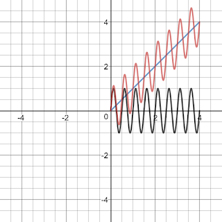
( x(t), y(t) ) = ( t,  t + sin(2*(2*pi*t) ) for ( 0 <= t <= 4)

In blue you see the line ( x(t), y(t) ) = (t, t). In black you see the squiggle (x(t),y(t)) = (t, sin(2*(2*pi*t))). In red you see both combined: (x(t),y(t)) = (t, t + sin(2*(2*pi*t))). Note that in the combined version, x should not move faster than in the separate versions so for this reason the x component is not changed.

What would the tilted squiggle look like if we oscillated in x direction instead of the y direction? Let's try to find out: (x(t), y(t)) = (t + sin(2*(2*pi*t)), t).

In blue you see the line ( x(t), y(t) )  = (t, t). In black you see the squiggle (x(t),y(t)) = (sin(2*(2*pi*t)), t)). In red you see the combination (x(t),y(t)) = (t + sin(2*(2*pi*t)), t).

What happens if we squiggle in both x and y direction simultaneously?
(x(t),y(t)) = (t + sin(4*pi*t), t + sin(4*pi*t) ).

 Ahm... what? That is a disappointment. Surely that can't be right? Right!? But actually this is correct. If you squiggle left and right in perfect sync with squiggling up and down you get a straight line. Things change quite drastically however, if you don't do it in perfect sync. Let's try some examples where we squiggle up and down with the same speed, but different phase:

(x(t),y(t)) = (t + sin(4*pi*t), t + sin(4*pi*t + pi) )

(x(t),y(t)) = (t + sin(4*pi*t), t + sin(4*pi*t + pi/2) )

(x(t),y(t)) = (t + sin(4*pi*t), t + sin(4*pi*t + pi/4) )

What if we squiggled in x and y direction with different frequencies instead? By playing with frequency and phase you can get some really intricate results, e.g.

(x(t),y(t)) = (t + sin(2pi*t - (2*pi/10)), t + sin(3pi*t + pi/3) )

Tapering

With the parametric equations we have a lot of power at our hands to further transform the generated curves. Suppose we want the squiggle to widen as time progresses. We already knew we can widen the squigle by stretching it (multiplying it) with a constant. But now we want the widening to increase as time progresses, so instead of multiplying it with a constant, we want to multiply it with something that increases as time increases. Can you think of such a thing? The answer is quite obvious once you know it: we can multiply it with time t itself! (Or some scaled and shifted version of it). Let's try out the idea on our tilted squiggle. We'll add tapering by multiplying the squiggly parts (the sines) with t/4:

(x(t),y(t)) = (t + t/4*sin(4*pi*t), t + t/4*sin(4*pi*t + pi) )

If instead of linear tapering you wanted quadratic tapering, you would multiply with a quadratic tapering function (here I've increased the domain of t to 0 <= t <= 8 to better show the quadratic shape). (x(t), y(t)) = (t + t^2/16*sin(4*pi*t), t + t^2/16*sin(4*pi*t + pi))

Bending squiggles

There's really no limit to what you can do. Suppose I wanted to take the linearly tapered squiggle and bend it around a circle with radius 10. Remember that we tilted the squiggled line by adding a horizontal version to a tilted line. Perhaps we can do the same with a circle? The parametric equation for a circle with radius 10 is (x(t),y(t)) = ( 10*sin(t), 10*cos(t) ) for 0 <= t <= 2pi. As before we can reparametrize the equation to make the bounds compatible with the tapered squiggle. We want to vary t from 0 to 4 instead of from 0 to 2pi. This means that we introduce a new parameter q = (4*t/(2pi)), which implies t = (2pi)*q/4. Then indeed 0 <= t <= 2pi, so 0 <= q*(2pi)/4 <= 2pi, so 0 <= q <= 4.
The circle equation therefore becomes (x(q), y(q)) = (10*sin(2pi*q/4), 10*cos(2pi*q/4)). And we can now just replace symbol q with symbol t again (technically this is a different t than before, one that now has compatible bounds) to get (x(t), y(t) ) = (10*sin(2pi*t/4), 10*cos(2pi*t/4)).

Let's see what happens if we add the tapered squiggle to this circle instead (I've increased the number of squiggles to make the effect more obvious:

(x(t),y(t)) = (10*sin(2*pi*t/4) + t/4*sin(16*pi*t), 10*cos(2*pi*t/4) + t/4*sin(16*pi*t + pi) )

.

Can you think of a way to make a squiggly spiral instead of a squiggly circle now (hint: something with the radius of the circle being time dependent)? Or how would you bend it over a quarter circle instead of a complete circle (hint: something with time rescaling of the circle equation)?

Polar equations

You may think by now that you are an absolute master in everything related to parametric equations, but nothing could be further from the truth. Many types of squiggles exist that we cannot easily construct with the insights presented before. One such type of squiggle is that which involves intricate circular movements (think mandala's). And for those types of squiggles, it's usually easier to think in terms of so-called polar equations. Polar equations can easily be translated to parametric equations so the insights from the previous paragraphs are not be lost.

So how are polar equations described? They are described as a variation of radius in function of the angle: radius = r(phi). Such equation can be translated to a parametric equation as follows: (x, y) =  (radius*cos(phi), radius*sin(phi)).

Suppose you have a constant radius 1 for all angles phi. What curve do you get? A circle.
r = 1

To convert r = 1 in polar form into parametric form, we can use the formulas given above:
x = r.sin(phi) = sin(phi)
y = r.cos(phi) = cos(phi)

Since phi is just a parameter that varies e.g. from 0 to 2pi, we can rename it to t, also varying from 0 to 2pi (or we can perform a substitution phi = 2pi*t, so that the range of t now varies between 0 and 1 instead of 0 and 2pi).

How can be make this a squiggly circle? By varying the radius as phi changes. We want the radius to oscillate as phi changes: we can again use sine, triangular or sawtooth waves, e.g.

r = sin(6*phi) + 2

In parametric equations, this would be:
x = r*sin(phi) = (sin(6*phi) + 2)*sin(phi)
y = r*cos(phi) = (sin(6*phi) + 2)*cos(phi)

Or a spiral with r(phi) = 0.1*phi/(2*pi), which in parametric equations becomes
(x(phi), y(phi) ) = (r*sin(phi), r*cos(phi)) = (0.1*phi/(2*pi)sin(phi), 0.1*phi/(2*pi)cos(phi))

Or maybe you want to scribble something more chaotic like r = cos(0.95*phi/8) (for 0 <= phi <= 40*pi):

Or something more aesthetic like this rose? r = phi + 2*sin(2*pi*phi) + 4*cos(2*pi*theta)

Bezier curves

(image courtesy of https://plus.maths.org/content/bridges-string-art-and-bezier-curves)

Nothing special here. With everything you know already some equations should suffice. 

• Bezier curve segment specified with 2 control points (i.e. a line between known points (x1,y1) and (x2, y2)): (x(t), y(t)) = (x1 - t(x2- x1), y1 - t(y2-y1)) for 0 <= t <= 1
• Bezier curve segment specified with 3 control points (x1, y1), (x2, y2) and (x3, y3): (x(t), y(t)) = ((1-t)^2*x1 + 2(1-t)t*x1 + t^2*x2, (1-t)^2*y1 + 2(1-t)t*y1 + t^2*y2)
• You can concatenate several 3-control Bezier curve segments to form larger curves. You can also create higher order Bezier curve segments using more than 3 control points. The formulas can be found on wikipedia.

Concatenation and periodization of parametric curves

In some environments (like in supercollider Synths) it is difficult to perform if-then-else. The lack of if-then-else makes it hard to concatenate parametric equation segments. Supercollider luckily offers the Select UGen which allows one to fake if-then-else by evaluating all branches and selecting results from only one of them.

As an alternative, one can also concatenate the curve segments mathematically. This is explained in the paper "Single equation without inequalities to represent a composite curve" by "E. Chicurel-Uziel", available from Elsevier's Computer Aided Geometric Design (worth reading!).

I won't repeat the complete paper here, but the techniques in the paper are directly applicable to our use cases. The basic idea is to define a step-function that can be used as a "switch" to switch on or off a certain parametric equation in a given interval. This can be combined with retiming of the parametric curve (i.e. substite all "t" with "t-a" to delay the curve with a time units) to concatenate different curves into one bigger curve. They also describe a way to make non-periodic function segments periodic both for cartesian and polar coordinates. 

Full explanation falls outside the scope of this blog post (maybe in a later one?), but if you understood everything so far the article itself is not a lot more difficult.

As a supercollider-only alternative, one may also sequence the different curve segments using patterns.

Conclusion

Note that so far we've barely scratched the possibilities. It's not so difficult to imagine how tons of stuff is possible by cleverly combining techniques and by introducing other functions besides polynomials and sines. Feel free to post your best squiggles in the comments section! 

With some techniques under our belt, let's now tackle the implementation in supercollider. As stated before, the aim is to replace MouseX and MouseY with pre-programmed squiggles.

Implementation in supercollider

In the previous sections we've always used an abstract parameter t (or "time") and this parameter t always varied from some lower bound (usually 0) to some upper bound (often 1 or 2pi). Where will this parameter come from in supercollider?

The simplest way of creating a parameter that goes from some lower bound to an upper bound is to use a sawtooth wave. If we use only one period of the sawtooth wave, we generate the complete squiggle exactly once. But if we use multiple periods, the same squiggle is generated multiple times as well.

If instead of a sawtooth wave we use a triangular wave, then we always generated the squiggle from beginning to end, followed by the same squiggle in reverse (time counts down again as the triangle goes down again).

Let's start by taking a synthdef that sounds somewhat interesting with a MouseX and a MouseY.

Run it in supercollider and notice how squiggling with the mouse creates some interesting effects.

Now choose a squiggle. I chose r = sin(5*phi) + 2 in polar coordinates (very similar to the 2nd figure in the section on polar coordinates, only 5 lobes instead of 6). Here's the supercollider implementation. It also displays a scope which, if you put it in X/Y mode will show you the squiggle as it is generated and executed.

By changing "speed" you can traverse the 2d space faster/more slowly, and by changing "rotations" you can traverse the 2d space partially/multiple times (i.e. multiple complete rotations). The "rotations" parameter has no effect on perfectly cyclic squiggles like the flower shape, but it would have an important effect on non-cyclic squiggles, like a spiral.

The only thing that needs to be changed to switch to a different squiggle in polar coordinates is the line that defines "commonpart" and the min and max x and y values of the generated squiggle (and of course speed and rotations can be set to personal taste).

Applying the theory from this post yields us:

However, the following - technically flawed - version actually sounds better... so I will keep it here as well. The mistake in case you are wondering is in confusing the sin operation with the SinOsc oscillator.

The example below can be downloaded from http://sccode.org/1-57x

And here's another example with the quadratically tapered squiggle (x(t), y(t)) = (t + t^2/16*sin(4*pi*t), t + t^2/16*sin(4*pi*t + pi)):

And of course, nothing stops you from also animating other parameters. There's literally no reason why e.g. you couldn't turn parameter speed into a squiggle as well.

Finally here's a longer example that combines multiple squiggles together and also visualizes them while they are being generated. While implementing this example, it became clear that there are many (MANY!) possible pitfalls you can fall into. But hey... at least the maths never lies.

First the Desmona design:

Next the source code (get it from http://sccode.org/1-57z )

And finally a screenshot of the thing running:

Have fun!